Tutorial

This is a tutorial for the momi package. You can run the ipython notebook that created this tutorial at docs/tutorial.ipynb.

To get started, import the momi package:

import momi

Some momi operations can take awhile complete, so it is useful to turn on status monitoring messages to check that everything is running normally. Here, we output logging messages to the file tutorial.log.

import logging
logging.basicConfig(level=logging.INFO,
                    filename="tutorial.log")

Constructing a demographic history

Use DemographicModel to construct a demographic history. Below, we set the diploid effective size N_e=1.2e4, the generation time gen_time=29 years per generation, and mutation rate muts_per_gen=1.25e-8 per base per generation.

model = momi.DemographicModel(N_e=1.2e4, gen_time=29,
                              muts_per_gen=1.25e-8)

Use DemographicModel.add_leaf to add sampled populations. Below we add 3 populations: YRI, CHB, and NEA. The archaic NEA population is sampled t=5e4 years ago. The YRI population has size N=1e5, while the CHB population is initialized to have size N=1e5 and growth rate g=5e-4 per year (NEA starts at the default size 1.2e4).

# add YRI leaf at t=0 with size N=1e5
model.add_leaf("YRI", N=1e5)
# add  CHB leaf at t=0, N=1e5, growing at rate 5e-4 per unit time (year)
model.add_leaf("CHB", N=1e5, g=5e-4)
# add NEA leaf at 50kya and default N
model.add_leaf("NEA", t=5e4)

Demographic events are added to the model by the methods DemographicModel.set_size and DemographicModel.move_lineages. DemographicModel.set_size is used to change population size and growth rate, while DemographicModel.move_lineages is used for population split and admixture events.

# stop CHB growth at 10kya
model.set_size("CHB", g=0, t=1e4)

# at 45kya CHB receive a 3% pulse from GhostNea
model.move_lineages("CHB", "GhostNea", t=4.5e4, p=.03)
# at 55kya GhostNea joins onto NEA
model.move_lineages("GhostNea", "NEA", t=5.5e4)

# at 80 kya CHB goes thru bottleneck
model.set_size("CHB", N=100, t=8e4)
# at 85 kya CHB joins onto YRI; YRI is set to size N=1.2e4
model.move_lineages("CHB", "YRI", t=8.5e4, N=1.2e4)

# at 500 kya YRI joins onto NEA
model.move_lineages("YRI", "NEA", t=5e5)

Note that events can involve other populations aside from the 3 sampled populations YRI, CHB, and NEA. Unsampled populations are also known as “ghost populations”. In this example, CHB receives a small amount of admixture from a population “GhostNea”, which splits off from NEA at an earlier date.

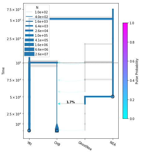
Plotting a demography

momi relies on matplotlib for plotting. In a notebook, first call %matplotlib inline to enable matplotlib, then you can use DemographyPlot to create a plot of the demographic model.

%matplotlib inline

yticks = [1e4, 2.5e4, 5e4, 7.5e4, 1e5, 2.5e5, 5e5, 7.5e5]

fig = momi.DemographyPlot(
    model, ["YRI", "CHB", "GhostNea", "NEA"],
    figsize=(6,8),
    major_yticks=yticks,
    linthreshy=1e5, pulse_color_bounds=(0,.25))

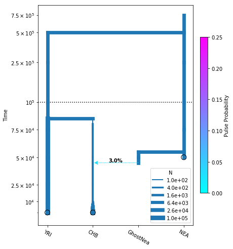
Note the user needs to specify the order of all populations (including ghost populations) along the x-axis.

The argument linthreshy is useful for visualizing demographic events at different scales. In our example, the split time of NEA is far above the other events. Times below linthreshy are plotted on a linear scale, while times above it are plotted on a log scale.

Reading and simulating data

In this section we demonstrate how to read in data from a VCF file. We start by simulating a dataset so that we can read it in later.

Simulating data

Use DemographicModel.simulate_vcf to simulate data (using msprime) and save the resulting dataset to a VCF file.

Below we simulate a dataset of diploid individuals, with 20 “chromosomes” of length 50Kb, with a recombination rate of 1.25e-8.

recoms_per_gen = 1.25e-8
bases_per_locus = int(5e5)
n_loci = 20
ploidy = 2

# n_alleles per population (n_individuals = n_alleles / ploidy)
sampled_n_dict = {"NEA":2, "YRI":4, "CHB":4}

# create data directory if it doesn't exist
!mkdir -p tutorial_datasets/

# simulate 20 "chromosomes", saving each in a separate vcf file
for chrom in range(1, n_loci+1):
      model.simulate_vcf(
            f"tutorial_datasets/{chrom}",
            recoms_per_gen=recoms_per_gen,
            length=bases_per_locus,
            chrom_name=f"chr{chrom}",
            ploidy=ploidy,
            random_seed=1234+chrom,
            sampled_n_dict=sampled_n_dict,
            force=True)

We saved the datasets in tutorial_datasets/$chrom.vcf.gz. Accompanying tabix and bed files are also created.

!ls tutorial_datasets/

10.bed         14.bed         18.bed         2.bed         6.bed
10.vcf.gz      14.vcf.gz      18.vcf.gz      2.vcf.gz      6.vcf.gz
10.vcf.gz.tbi  14.vcf.gz.tbi  18.vcf.gz.tbi  2.vcf.gz.tbi  6.vcf.gz.tbi
11.bed         15.bed         19.bed         3.bed         7.bed
11.vcf.gz      15.vcf.gz      19.vcf.gz      3.vcf.gz      7.vcf.gz
11.vcf.gz.tbi  15.vcf.gz.tbi  19.vcf.gz.tbi  3.vcf.gz.tbi  7.vcf.gz.tbi
12.bed         16.bed         1.bed          4.bed         8.bed
12.vcf.gz      16.vcf.gz      1.vcf.gz       4.vcf.gz      8.vcf.gz
12.vcf.gz.tbi  16.vcf.gz.tbi  1.vcf.gz.tbi   4.vcf.gz.tbi  8.vcf.gz.tbi
13.bed         17.bed         20.bed         5.bed         9.bed
13.vcf.gz      17.vcf.gz      20.vcf.gz      5.vcf.gz      9.vcf.gz
13.vcf.gz.tbi  17.vcf.gz.tbi  20.vcf.gz.tbi  5.vcf.gz.tbi  9.vcf.gz.tbi

Read in data from vcf

Now we read in the datasets we just simulated.

The first step is to create a mapping from individuals to populations. We save this mapping to a text file whose first column is for individuals and second column is for populations.

# a dict mapping samples to populations
ind2pop = {}
for pop, n in sampled_n_dict.items():
    for i in range(int(n / ploidy)):
        # in the vcf, samples are named like YRI_0, YRI_1, CHB_0, etc
        ind2pop["{}_{}".format(pop, i)] = pop

with open("tutorial_datasets/ind2pop.txt", "w") as f:
    for i, p in ind2pop.items():
        print(i, p, sep="\t", file=f)

!cat tutorial_datasets/ind2pop.txt

NEA_0   NEA
YRI_0   YRI
YRI_1   YRI
CHB_0   CHB
CHB_1   CHB

Compute allele counts

The next step is to compute the allele counts for each VCF separately. To do this, use the shell command python -m momi.read_vcf $VCF $IND2POP $OUTFILE --bed $BED:

%%sh
for chrom in `seq 1 20`;
do
    python -m momi.read_vcf \
           tutorial_datasets/$chrom.vcf.gz tutorial_datasets/ind2pop.txt \
           tutorial_datasets/$chrom.snpAlleleCounts.gz \
           --bed tutorial_datasets/$chrom.bed
done

The --bed flag specifies a BED accessible regions file; only regions present in the BED file are read from the VCF. The BED file also determines the length of the data in bases. If no BED file is specified, then all SNPs are read, and the length of the data is set to unknown.

You should NOT use the same BED file across multiple VCF files, and should ensure your BED files do not contain overlapping regions. Otherwise, regions will be double-counted when computing the length of the data. You can use tabix to split a single BED file into multiple non-overlapping files.

By default ancestral alleles are read from the INFO AA field (SNPs missing this field are skipped) but this behavior can be changed by setting the flags --no_aa or --outgroup.

Use the --help flag to see more command line options, and see also the documentation for SnpAlleleCounts.read_vcf, which provides the same functionality within Python.

Extract combined SFS

Use python -m momi.extract_sfs $OUTFILE $NBLOCKS $COUNTS... from the command line to combine the SFS across multiple files, and split the SFS into a number of equally sized blocks for jackknifing and bootstrapping.

%%sh
python -m momi.extract_sfs tutorial_datasets/sfs.gz 100 tutorial_datasets/*.snpAlleleCounts.gz

Use the --help flag to see the command line options, and see also the documentation for SnpAlleleCounts.concatenate and SnpAlleleCounts.extract_sfs which provide the same functionality within Python.

Read SFS into Python

Finally, read the SFS file into Python with Sfs.load:

sfs = momi.Sfs.load("tutorial_datasets/sfs.gz")

Inference

In this section we will infer a demography for the data we simulated. We will start by fitting a sub-demography on CHB and YRI, and then iteratively build on this model, by adding the NEA population and also additional parameters and events.

An initial model for YRI and CHB

We will start by fitting a simplifed model without admixture. Use DemographicModel() to initialize it as before:

no_pulse_model = momi.DemographicModel(
    N_e=1.2e4, gen_time=29, muts_per_gen=1.25e-8)

Note that muts_per_gen is optional, and can be omitted if unknown, but specifying it provides extra power to the model.

Use DemographicModel.set_data to add data to the model for inference:

no_pulse_model.set_data(sfs)

To add parameters to the model, use DemographicModel.add_size_param, DemographicModel.add_time_param, DemographicModel.add_growth_param, and DemographicModel.add_pulse_param.

Below we define parameters for the CHB size, the CHB growth rate, and the CHB-YRI split time:

# random initial value
no_pulse_model.add_size_param("n_chb")
# initial value 0; user-specified lower,upper bounds
no_pulse_model.add_growth_param("g_chb", 0, lower=-1e-3, upper=1e-3)
# random initial value; user-specified lower bound
no_pulse_model.add_time_param("t_chb_yri", lower=1e4)

Demographic events can be added similarly as before. Parameters are specified by name (string), while constants are specified as numbers (float).

no_pulse_model.add_leaf("CHB", N="n_chb", g="g_chb")
no_pulse_model.add_leaf("YRI", N=1e5)
no_pulse_model.set_size("CHB", t=1e4, g=0)
no_pulse_model.move_lineages("CHB", "YRI", t="t_chb_yri", N=1.2e4)

Use DemographicModel.optimize to search for the MLE. It is a thin wrapper around scipy.optimize.minimize and accepts similar arguments.

no_pulse_model.optimize(method="TNC")

/home/jack/miniconda3/envs/momi2-conda-nomkl/lib/python3.6/site-packages/autograd/numpy/numpy_vjps.py:444: FutureWarning: Using a non-tuple sequence for multidimensional indexing is deprecated; use `arr[tuple(seq)]` instead of `arr[seq]`. In the future this will be interpreted as an array index, `arr[np.array(seq)]`, which will result either in an error or a different result.
  return lambda g: g[idxs]

            fun: 0.003629860012261981
            jac: array([-6.52603508e-06, -3.58838649e-02, -8.63552150e-10])
  kl_divergence: 0.003629860012261981
 log_likelihood: -30444.557113445273
        message: 'Converged (|f_n-f_(n-1)| ~= 0)'
           nfev: 56
            nit: 24
     parameters: ParamsDict({'n_chb': 14368074.379920935, 'g_chb': 0.000997783661801449, 't_chb_yri': 114562.32318043888})
         status: 1
        success: True
              x: array([1.64805192e+01, 9.97783662e-04, 1.04562323e+05])

The default optimization method is method="TNC" (truncated Newton conjugate). This is very accurate but can be slow for large models; for large models, method="L-BFGS-B" is a good choice.

We can print the inferred parameter values with DemographicModel.get_params:

no_pulse_model.get_params()

ParamsDict({'n_chb': 14368074.379920935, 'g_chb': 0.000997783661801449, 't_chb_yri': 114562.32318043888})

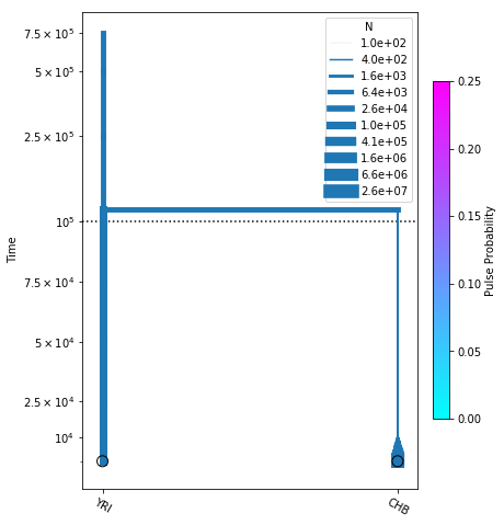
and we can plot the inferred demography as before:

# plot the model
fig = momi.DemographyPlot(no_pulse_model, ["YRI", "CHB"],
                          figsize=(6,8), linthreshy=1e5,
                          major_yticks=yticks,
                          pulse_color_bounds=(0,.25))

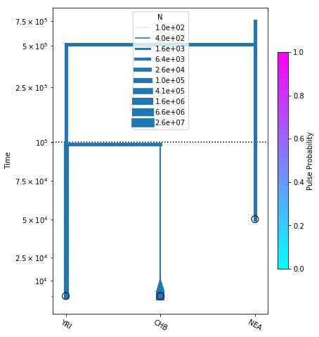
Adding NEA to the existing model

Now we add in the NEA population, along with a parameter for its split time t_anc. We use the keyword lower_constraints to require that t_anc > t_chb_yri.

no_pulse_model.add_leaf("NEA", t=5e4)
no_pulse_model.add_time_param("t_anc", lower=5e4, lower_constraints=["t_chb_yri"])
no_pulse_model.move_lineages("YRI", "NEA", t="t_anc")

We search for the new MLE and plot the inferred demography:

no_pulse_model.optimize()

fig = momi.DemographyPlot(
    no_pulse_model, ["YRI", "CHB", "NEA"],
    figsize=(6,8), linthreshy=1e5,
    major_yticks=yticks)

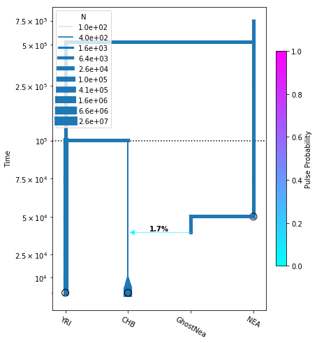
Build a new model adding NEA->CHB

Now we create a new DemographicModel, by copying the previous model and adding a NEA->CHB migration arrow.

add_pulse_model = no_pulse_model.copy()
add_pulse_model.add_pulse_param("p_pulse", upper=.25)
add_pulse_model.add_time_param(
    "t_pulse", upper_constraints=["t_chb_yri"])

add_pulse_model.move_lineages(
    "CHB", "GhostNea", t="t_pulse", p="p_pulse")

add_pulse_model.add_time_param(
    "t_ghost", lower=5e4,
    lower_constraints=["t_pulse"], upper_constraints=["t_anc"])
add_pulse_model.move_lineages(
    "GhostNea", "NEA", t="t_ghost")

It turns out this model has local optima, so we demonstrate how to fit a few independent runs with different starting parameters.

Use DemographicModel.set_params to set new parameter values to start the search from. If a parameter is not specified and randomize=True, a new value will be randomly sampled for it.

results = []
n_runs = 3
for i in range(n_runs):
    print(f"Starting run {i+1} out of {n_runs}...")
    add_pulse_model.set_params(
        # parameters inherited from no_pulse_model are set to their previous values
        no_pulse_model.get_params(),
        # other parmaeters are set to random initial values
        randomize=True)

    results.append(add_pulse_model.optimize(options={"maxiter":200}))

# sort results according to log likelihood, pick the best (largest) one
best_result = sorted(results, key=lambda r: r.log_likelihood)[-1]

add_pulse_model.set_params(best_result.parameters)
best_result

Starting run 1 out of 3...
Starting run 2 out of 3...
Starting run 3 out of 3...

            fun: 0.006390407169686503
            jac: array([ 3.86428996e-08, -8.26898179e-02,  4.63629649e-13, -7.35845677e-14,
       -2.69540750e-07, -2.98321219e-07,  1.46475502e-08])
  kl_divergence: 0.006390407169686503
 log_likelihood: -60986.74341175791
        message: 'Converged (|f_n-f_(n-1)| ~= 0)'
           nfev: 78
            nit: 21
     parameters: ParamsDict({'n_chb': 11824540.526927987, 'g_chb': 0.001, 't_chb_yri': 100366.89310119499, 't_anc': 524505.2984953767, 'p_pulse': 0.017396498328507242, 't_pulse': 39601.33887335411, 't_ghost': 50387.43446019594})
         status: 1
        success: True
              x: array([ 1.62856876e+01,  1.00000000e-03,  9.03668931e+04,  4.24138405e+05,
       -4.03393674e+00, -4.28160158e-01, -7.10966453e+00])

# plot the model
fig = momi.DemographyPlot(
    add_pulse_model, ["YRI", "CHB", "GhostNea", "NEA"],
    linthreshy=1e5, figsize=(6,8),
    major_yticks=yticks)
# put legend in upper left corner
fig.draw_N_legend(loc="upper left")

<matplotlib.legend.Legend at 0x7fdb6ff738d0>

Statistics of the SFS

Here we discuss how to compute statistics of the SFS, for evaluating the goodness-of-fit of our models, and for estimating the mutation rate.

Goodness-of-fit

Use SfsModelFitStats to see how well various statistics of the SFS fit a model, via the block-jackknife.

Below we create an SfsModelFitStats to evaluate the goodness-of-fit of the no_pulse_model.

no_pulse_fit_stats = momi.SfsModelFitStats(no_pulse_model)

One important statistic is the f4 or “ABBA-BABA” statistic for detecting introgression (Patterson et al 2012).

In the absence of admixture f4(YRI, CHB, NEA, AncestralAllele) should be 0, but for our dataset it will be negative due to the NEA->CHB admixture.

Use SfsModelFitStats.f4 to compute f4 stats. For the no-pulse model, we see that f4(YRI, CHB, NEA, AncestralAllele) is indeed negative.

print("Computing f4(YRI, CHB, NEA, AncestralAllele)")
f4 = no_pulse_fit_stats.f4("YRI", "CHB", "NEA", None)

print("Expected = {}".format(f4.expected))
print("Observed = {}".format(f4.observed))
print("SD = {}".format(f4.sd))
print("Z(Expected-Observed) = {}".format(f4.z_score))

Computing f4(YRI, CHB, NEA, AncestralAllele)
Expected = 6.938893903907228e-18
Observed = -0.003537103263299063
SD = 0.0017511821832936283
Z(Expected-Observed) = -2.0198373972983648

The related f2 and f3 statistics are also available via SfsModelFitStats.f2 and SfsModelFitStats.f3.

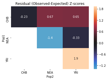
Another method for evaluating model fit is SfsModelFitStats.all_pairs_ibs, which computes the probability that two random alleles are the same, for every pair of populations:

no_pulse_fit_stats.all_pairs_ibs()

	Pop1	Pop2	Expected	Observed	Z
0	YRI	YRI	0.699637	0.706936	1.924912
1	NEA	NEA	0.732753	0.720787	-1.388584
2	CHB	NEA	0.545176	0.548234	0.668636
3	CHB	YRI	0.694800	0.697731	0.651155
4	NEA	YRI	0.545176	0.543831	-0.334112
5	CHB	CHB	0.965634	0.964595	-0.231728

Finally, the method SfsModelFitStats.tensor_prod can be used to compute very general statistics of the SFS (specifically, linear combinations of tensor-products of the SFS). See the documentation for more details.

Limitations of SfsModelFitStats

Note the SfsModelFitStats class above has some limitations. First, it computes goodness-of-fit for the SFS without any missing data; all entries with missing samples are removed. For datasets with many individuals and pervasive missingness, this can result in most or all of the data being removed.

In such cases you can specify to use the SFS restricted to a smaller number of samples; then all SNPs with at least that many of non-missing individuals will be used. For example,

no_pulse_fit_stats = momi.SfsModelFitStats(
    no_pulse_model, {"YRI": 2, "CHB": 2, "NEA": 2})

will compute statistics for the SFS restricted to 2 samples per population.

The second limitation of SfsModelFitStats is that it ignores the mutation rate – it only fits the SFS normalized to be a probability distribution. However, see the next subsection on how to evaluate the total number of mutations in the data.

Estimating mutation rate

To evaluate the total number of mutations in the data, e.g. to fit the mutation rate, use the method DemographicModel.fit_within_pop_diversity, which computes the within-population nucleotide diversity, i.e. the heterozygosity of a random individual in that population assuming Hardy-Weinberg Equilibrium:

no_pulse_model.fit_within_pop_diversity()

	Pop	EstMutRate	JackknifeSD	JackknifeZscore
0	CHB	1.283114e-08	1.624236e-09	0.203875
1	YRI	1.215218e-08	1.571356e-10	-2.213517
2	NEA	1.301250e-08	4.018888e-10	1.275228

This method returns a dataframe giving estimates for the mutation rate. Note that there is an estimate for each population – these estimates are non-independent estimates for the same value, just computed in different ways (by computing the expected to observed heterozygosity for each population separately). These estimates account for missingness in the data; it is fine to use it on datasets with large amounts of missingness.

Since we initialized our model with muts_per_gen=1.25e-8, the method also returns a Z-value for the residuals of the estimated mutation rates.

Bootstrap confidence intervals

Use Sfs.resample to create bootstrap datasets by resampling blocks of the SFS.

To generate confidence intervals, we can refit the model on the bootstrap datasets and examine the quantiles of the re-inferred parameters. Below we do this for a very small number of bootstraps and a simplified fitting procedure. In practice you would want to generate hundreds of bootstraps on a cluster computer.

n_bootstraps = 5
# make copies of the original models to avoid changing them
no_pulse_copy = no_pulse_model.copy()
add_pulse_copy = add_pulse_model.copy()

bootstrap_results = []
for i in range(n_bootstraps):
    print(f"Fitting {i+1}-th bootstrap out of {n_bootstraps}")

    # resample the data
    resampled_sfs = sfs.resample()
    # tell models to use the new dataset
    no_pulse_copy.set_data(resampled_sfs)
    add_pulse_copy.set_data(resampled_sfs)

    # choose new random parameters for submodel, optimize
    no_pulse_copy.set_params(randomize=True)
    no_pulse_copy.optimize()
    # initialize parameters from submodel, randomizing the new parameters
    add_pulse_copy.set_params(no_pulse_copy.get_params(),
                              randomize=True)
    add_pulse_copy.optimize()

    bootstrap_results.append(add_pulse_copy.get_params())

Fitting 1-th bootstrap out of 5
Fitting 2-th bootstrap out of 5
Fitting 3-th bootstrap out of 5
Fitting 4-th bootstrap out of 5
Fitting 5-th bootstrap out of 5

We can visualize the bootstrap results by overlaying them onto a single plot.

# make canvas, but delay plotting the demography (draw=False)
fig = momi.DemographyPlot(
    add_pulse_model, ["YRI", "CHB", "GhostNea", "NEA"],
    linthreshy=1e5, figsize=(6,8),
    major_yticks=yticks,
    draw=False)

# plot bootstraps onto the canvas in transparency
for params in bootstrap_results:
    fig.add_bootstrap(
        params,
        # alpha=0: totally transparent. alpha=1: totally opaque
        alpha=1/n_bootstraps)

# now draw the inferred demography on top of the bootstraps
fig.draw()
fig.draw_N_legend(loc="upper left")

<matplotlib.legend.Legend at 0x7fdb702e54e0>

Other features

Stochastic gradient descent

For large models, it can be useful to perform stochastic optimization: instead of computing the full likelihood at every step, we use a random subset of SNPs at each step to estimate the likelihood gradient. This is especially useful for rapidly searching for a reasonable starting point, from which full optimization can be performed.

DemographicModel.stochastic_optimize implements stochastic optimization with the ADAM algorithm. Setting svrg=n makes the optimizer use the full likelihood every n steps which can lead to better convergence (see SVRG).

The cell below performs 10 steps of stochastic optimization, using 1000 random SNPs per step, and computing the full likelihood every 3 iterations.

add_pulse_copy.stochastic_optimize(
    snps_per_minibatch=1000, num_iters=10, svrg_epoch=3)

            fun: 3.5684750877096234
            jac: array([ 2.16057690e-06, -2.30524330e-03,  2.41528617e-07, -1.54878487e-07,
        1.07274014e-03, -3.48843607e-10, -2.21603171e-09])
 log_likelihood: 3.5684750877096234
        message: 'Maximum number of iterations reached'
            nit: 9
     parameters: ParamsDict({'n_chb': 17322702.843983896, 'g_chb': -0.001, 't_chb_yri': 94934.93099677152, 't_anc': 515875.5851996526, 'p_pulse': 0.0008410052687267091, 't_pulse': 1081.016605046677, 't_ghost': 50008.16334495788})
        success: False
              x: array([ 1.66675285e+01, -1.00000000e-03,  8.49349310e+04,  4.20940654e+05,
       -7.08007127e+00, -4.46383757e+00, -1.09520024e+01])

Using functions of model parameters as demographic parameters

momi allows you to set a demographic parameter as a function of other model parameters.

For example, suppose we have a parameter t_div for the divergence time between 2 populations, and we would like to add a pulse event at time t_div / 2.

This can be achieved by passing a lambda function to move_lineages as follows:

model.move_lineages(pop1, pop2, t=lambda params: params.t_div / 2, p="p_mig")

The lambda function should take a single argument, params, which has all the defined parameters as attributes, e.g. params.t_div if you have defined a t_div parameter.

As another example, for a population that is exponentially growing since time t, we may parametrize the growth rate in terms of the population sizes at the beginning and end of the epoch:

model.add_leaf(pop, N="N_end", g=lambda params: np.log(params.N_end/params.N_start)/params.t_start)
model.set_size(pop, t="t_start", g=0)

This can be more numerically stable than parametrizing the growth rate directly (since small changes in the growth rate can cause very large changes in population sizes).

Some care is needed – momi internally uses autograd to compute gradients, so the function must be differentiable by autograd. Lambda functions to do simple arithmetic (as above) are fine, however more complex functions with variable assignments, or that call external methods, need some care, otherwise gradients will be wrong. It is highly recommended to read the autograd tutorial before using this feature.